
Anti-Aliasing
How to filter your shaders for better quality

Hi! Happy 2025. It’s been a long time (insert Dad joke about the new year here), but I’m back and ready to get some new tutorials done!
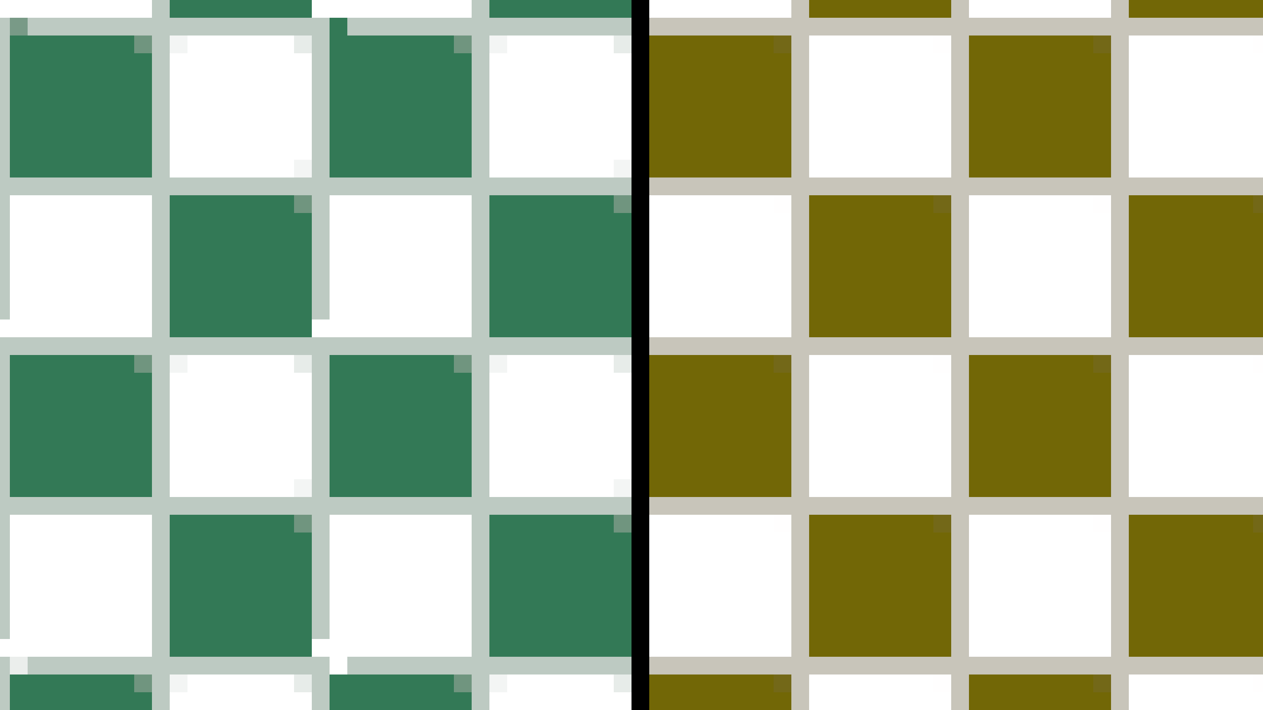
Today’s tutorial is about “analytic anti-aliasing”. Anti-aliasing is all about producing soft, natural-looking edges in your shaders. Here’s an image to illustrate the difference between an unfiltered and filtered checkerboard pattern:

Aliasing occurs when we have more color data than we can fit in the pixels. There are many ways to approach this. We could sample multiple points per pixel and average the results, but this can get expensive at higher resolutions.
In real life, cameras don’t have this issue because the pixel sensors receive zillions of photons to construct an image. They aren’t limited to one sample per pixel. We don’t have the luxury of simulating every photon, so we’ll have to find a way to approximate them.
Previously, we looked at a post-processing solution:
GM Shaders Mini: FXAA

Hi again! Today, we’re gonna take a look at the famous Fast Approximate Anti-Aliasing algorithm.
FXAA is a decent generalized solution, but it sometimes can cause unintended softening or other artifacts. There’s only so much that can be done with post-processing on the pixel colors. Let’s take a deeper look at the anti-aliasing process to expand our toolset!
Circle Example
The simplest example I could think of is drawing a circle. You could draw a circle by checking if a pixel is within the radius of the circle:
gl_FragColor = vec4(dist < rad);
This method introduces hard pixel edges. Alternatively, if you know (or can approximate) how close a pixel is to the edge, you can do a little sub-pixel gradient along that edge. This is easy to do with a circle because we already have the distance.
Here’s a close-up illustration of a circle with and without anti-aliasing:

The green dots represent the centers of each pixel. On the left side of the blue line, we simply check if the distance from the pixel to the center of the circle is within the radius. On the right side, we estimate how much of the pixel is within the radius. This could be calculated with complicated integrals of our function, but that is overkill!
Instead, a simple and effective approximation is to use the same distance value as earlier, but we blend from 0 to 1. So if the center of the pixel is on the radius line, we should expect 50% opacity. 50% roughly of the pixel is within the radius and 50% is out (it depends on the radius, but the effects are negligible). We should expect 100% opacity when the circle_radius - pixel_distance is greater than 0.5 pixels because it means that the radius is at the outside edge of the pixel. And we can expect 0% opacity when less than -0.5 pixels because that is the inside edge of the pixel.
So now all we need to do is make sure the distance is in pixel units and clamp the gradient to the [0, 1] range. We can divide by our “texel” scale to correct for
float gradient = clamp((radius - dist) / texel + 0.5, 0.0, 1.0);
Now the opacity can be set based on how close the pixel is to the edge, instead of just doing a distance check. I’ve put together a ShaderToy demo for more details here.
The best part is this method works with all Signed Distance Fields! All you need is to correct the scale of the distance field so that the 0 to 1 range matches the pixel scale. This method is perfect when you know the distance to the edges and the scale, but what if it’s not a perfect distance field? What if the gradient is inconsistent? A common example is with noise functions where some areas may have steep gradients while other spots can be flat. If this is your case, we’ll need to go further!
Derivative Methods
Let’s look at an example with a noise function. We can still get a gradient edge by doing: some_threshold - noise_value, which should generally return higher values as we get further from the edge, but not reliably. Noise is supposed to be unpredictable so it makes this more difficult.

If we try to use a constant scaling factor for the edges as on the left, some edges may be too soft while others could be too sharp. On the right, we are using the same method as before, but we’re calculating the gradient scale for every pixel, which leads to more consistent edges.
This is still an approximation, but it’s a step in the right direction and a big improvement on our previous method!
We can approximate the rate of change in the gradient by using derivatives. Definitely read my article on the topic if you haven’t yet because it’s important here!
GM Shaders Mini: Derivatives

Today, let's unpack “derivatives”. What are they for and how do they work?
The super simple solution here is to use fwidth() to calculate our scaling factor for us. The best part is that this works with most things out of the box:
//Approximate the smooth edges from any continuous function
float antialias_l1(float d)
{
    //Divide d by it's derivative width
    return clamp(0.5 +  d / fwidth(d), 0.0, 1.0);
}Note: We should be careful about potentially dividing by 0 here! You can do a quick check like so: float scale = width>0.0? 1.0/width : 1e7;
I like to take things a little further and calculate my fwidth manually with length. This produces better results at a slightly higher cost:
//Approximate the smooth edges from any continuous function
float antialias_l2(float d)
{
    //x and y derivatives
    vec2 dxy = vec2(dFdx(d), dFdy(d));
    //Get gradient width
    float width = length(dxy);
    //Calculate reciprocal scale (avoid division by 0!)
    float scale = width>0.0? 1.0/width : 1e7;
    //Normalize the gradient d with its scale
    return clamp(0.5 + 0.7 * scale * d, 0.0, 1.0);
}
This magic formula can blend the edges of just about any continuous function. It can handle a heavily distorted distance field, noise, and gradients of any sort. It’s only weakness is discontinuous functions since they break the derivatives. A distance expression like dist = floor(x/10.0) will not work because it jumps in steps and there is no gradient width to even approximate the scale with. If this is an issue for your shader needs, continue to the final step!
Edge Cases
There may be some instances where the partial derivatives computed with dFdx and dFdy are not good enough. Even something simple like a checkerboard can seem challenging to do, but there are two ways to solve it. You can either try to get rid of the discontinuities or you can calculate the derivative manually. A checkerboard can also be achieved with a formula like sin(x*PI)*sin(y*PI). This gives a continuous function that ranges from -1 to 1.
Also, sometimes 2x2 derivative chunks are not suitable for your shader or not precise enough. In these cases, you may have to calculate the derivatives manually.
Here’s an example of artifacts produced from coarse derivatives:
For these scenarios, we’ll use this function:
//For when the derivatives must be manually calculated
float antialias_l2_dxy(float d, vec2 dxy)
{
    //Get gradient width
    float width = length(dxy);
    //Calculate reciprocal scale (avoid division by 0!)
    float scale = width>0.0? 1.0/width : 1e7;
    //Normalize the gradient d with its scale
    return clamp(0.5 + 0.7 * scale * d, 0.0, 1.0);
}
Then we can generate our own partial derivatives like so:
//Get gradient (neighbors for manual derivatives)
float grad00 = grad(pos);
float grad10 = grad(pos+vec2(1,0));
float grad01 = grad(pos+vec2(0,1));
//Compute the xy derivatives
vec2 dxy = vec2(grad10, grad01) - grad00;Note: This is more expensive than the native derivative functions, which compute derivatives for nearly free! This is sampling our gradient function 3 times, so it should be used cautiously with larger or more complicated functions.
This manual derivative method can be used for anti-aliasing on multiple layers. A common example is with stripy patterns that have many edges:

Let’s say we have a stripe gradient “grad” that we want to range from 0 to 5 for 5 stripes. The edges separating the stripes, can be found with fract(grad) - 0.5, but fract is discontinuous and will break our derivatives. So for this, we want to calculate our derivatives on the original “grad” variable. I’ve put together a shader example here.
This same method can even be applied to pixel art anti-aliasing, but you do it on the x and y axes simultaneously using texture interpolation. I’m not going to go over the details here, but there are excellent resources out there on this topic if you’re interested!
Conclusion
To summarize, anti-aliasing is all about smoothly filtered edges without requiring rendering a higher resolution and downscaling. Today we covered the main 3 levels of filtering which can be used depending on the situation.
For simple shapes like circles, lines, squares, or Signed Distance Fields, it’s pretty trivial to generate smooth edges cheaply and there are very few reasons not to! It’s just a matter of matching the gradients to the pixel scale for consistent edge thickness.
Most other shaders will have more complicated shapes where we won’t have the luxury of knowing the exact distance to the nearest edge, but that’s okay. As long as we have a gradient that generally points towards the nearest edge, we can approximate the distance with derivatives (measuring the rates of change). The math can sound scary, but it’s usually not much more than fwidth(). Using the antialias_l2() function above should handle most situations without much work!
Finally, there are scenarios where you don’t even have a gradient or where gradient is discontinuous (has breaks in it). These cases require a little more work on a case-by-case basis, but many times you can rework it to make the gradient continuous or calculate the derivatives using a continuous, break-less version of the gradient. The derivatives only care about the rate of change and not the absolute value, so they can use independent formulas!
Hopefully, this guide gives you a good idea of how anti-aliasing actually works and how you can start to implement it into your own shaders! This is something every shader programmer should know because it’s useful all of the time. It’s better to produce smooth images from the start than to produce something rough and try to filter it after the fact.
Extras
“Exploring ways to mipmap alpha-tested textures” by Nikita Lisitsa (@lisyarus)
This is a nice overview on handling grass or vegetation textures in large-scale games. Grass textures tend to suffer when viewed from a distance because they are either too sharp (aliasing) or too blobby, but SDFs can be used to address that.
Here’s a reminder of why you should avoid using a lot of trig functions, especially atan2. Generally speaking, if you are converting a vector to an angle (with atan) and then back to a vector (with cos/sin) you’re probably overcomplicating something. Many operations can be applied directly to vectors and that’s how shaders are designed to operate! One atan2 here and there isn’t the end of the world, but it’s something to consider if you’re doing it a lot.
Alright, that’s it for now.
can you explain where the 0.7 comes from? i assume it's 1.0/sqrt(2) approximation, but can you explain specifically why that's desirable in this case?