Guest: Radiance Cascades
Part One: Introduction to Radiance Cascades
Hello again, this is Yaazarai (Alex) and I’m back for another tutorial on global illumination! The previous tutorial went over Radiosity which was a method for roughly approximating GI based on random per-pixel ray sampling. Its naive and extremely expensive to compute—casting some N amount of rays per pixel on the screen! That’s old news, Radiance Cascades is where its at, elegant, intuitive and simple in essence. Radiance Cascades is a new, noiseless, smart approach to both 2D and 3D global illumination created by Alexander Sannikov, a senior graphics programmer at Grinding Gear Games, the developers behind Path of Exile!
Before we get into the article I want to preface that this is Part One and a deep dive into the shader code behind this method won’t be until Part Two due to the complexity of introducing a the new subject.
Radiance Cascades is so effective because it casts finite amounts of rays in a special way to simulate an infinite amount of directions and how it does that is surprisingly simple (relatively speaking). So what does it look like, what can it look like and what’s possible? Let’s find out! First off is my demo which gets us up and running with a basic demonstration.
Even better, Radiance Cascades can do volumetrics (without SDFs, but that’s for another time). The very talented Mytino on Twitter has been able to integrate volumetrics through fluids, skybox integrals and directional light sources such as for bleeding sunlight into caves from the background.
Overview (TL;DR)
The most common way to simulate global illumination, is achieved by ray casting in random directions to see if we hit a light source or a shadow castor. This method requires casting loads of rays which can be quite expensive and the random noise has to be somehow filtered out (often with ghosting or oversoftening).
Radianace Cascades bypass the noise by taking a more structured approach. The first step is to cast a few short rays in a couple of directions (usually starting with 4). Then each successive pass increases the number of ray cast directions, while decreasing the Level Of Detail. 4x the number of rays and 1/4th resolution (half the width and half the height). This naturally creates more natural looking lighting with fine details up close and softer shadows in the distance (“penumbra”).
This algorithm isn’t perfect yet (with occasional light leaks and non-linear attenuation transitions), but it’s still being actively developed in the Graphics Programming discord, so this is well worth exploring!
Please note that this method is relatively new and still being actively researched and developed. The description provided herein is for a specific implementation of Radiance Cascades.
Penumbra Hypothesis
The penumbra hypothesis states: the penumbra of a shadow requires higher “linear resolution” closer to a light source and higher “angular resolution” further from the source. Linear resolution meaning number of pixels that make up the scene, and angular resolution meaning the number of rays directions for each pixel. The linear and angular resolution of a penumbra are inversely proportional.
Lets take the following example from the paper. Notice how the shadow becomes sharper closer to the light (yellow line) and blurrier (penumbra) further from the light.
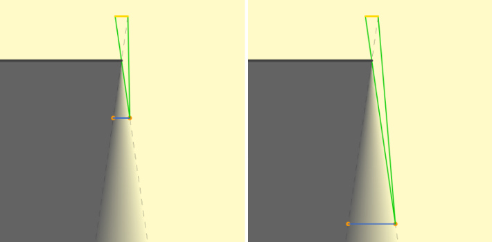
If we take any pixel on screen, the linear resolution is how close to that pixel we cast rays and the angular resolution is how many rays at that distance that are cast. Since the linear and angular resolutions are inversely proportional to one another we can take advantage of this property and decrease the spatial (linear) accuracy to which rays are cast from.
You can see this in action in the visualization from tmpvar’s playground for Radiance Cascades for more info and interactive demos. In orange we have the least amount of rays and the most amount of spatial points to cast rays from (higher spatial resolution), then 1/4x points and 4x rays in green and 1/4x points and 4x more rays in blue (higher angular resolution).
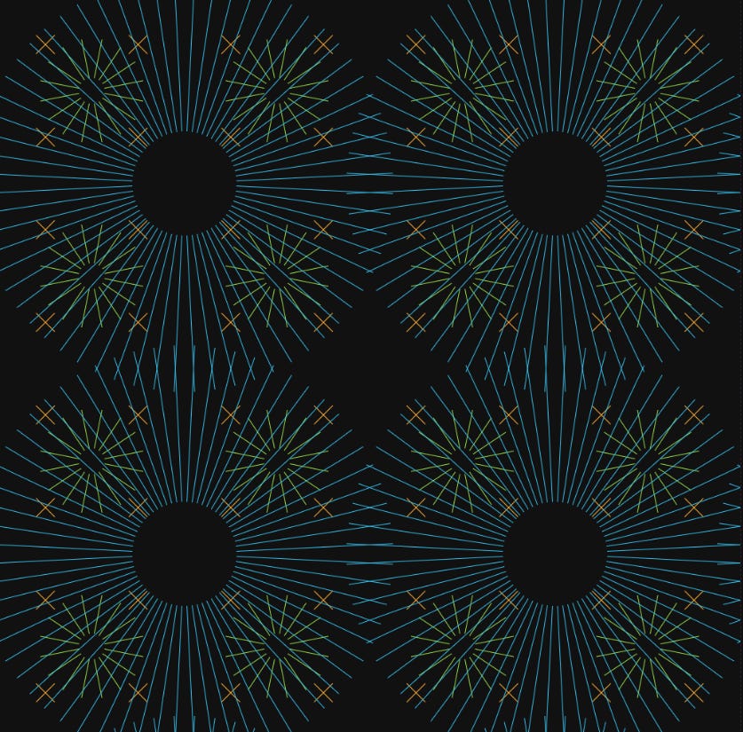
Here is an example of exaggerated rays converging to the approximated penumbra showing their linear and angular displacement across the penumbra using the same opaque half plane example. Less rays closer to the light source, more rays further from the light source just as the penumbra hypothesis predicts. Neat!
Figure 4.
Cascade Hierarchies
Now that we know how penumbras work we can start to resolve and approximate their properties with raymarching. This is done using cascade hierarchies acceleration structure and defining characteristic of “Radiance Cascades.” Cascades are a special memory layout which define how (distance and direction) and where (probe positions) we cast rays in the scene. However each of the pixels in the cascade actually store the radiance result of a ray that pixel represents. This layout is optimized to take advantage of the most intuitive part of the penumbra hypothesis: the inverse correlation between linear and angular resolution of penumbras.
Each cascade has some N number of probes and each probe has some R number of rays that it emits into the scene. Cascade0 has the most probes and the least rays and each following cascadeN has 1/4x as many probes (lower linear resolution) and 4x more rays (higher angular resolution). As seen again in figure 3 above.
The particular scaling 1/4x to 4x isn’t a hard requirement, but an optimal choice for 2D radiance cascades determined by Alexander Sannikov. Even better is that when using 4x scaling all cascades remain the same size in memory as well because the scaling between cascades is constant.

See figure 4 above. This is what those cascades look like in memory. From left to right we have cascade0 with 16x16 (256 total) probes, cascade1 with 8x8 (64 total), cascade2 4x4 (16 total) and finally cascade3 with 2x2 (4 total) probes.
From left to the right:
Cascade 0: 16 x 16 probes, 8 x 8 rays (256 total probes, 64 rays per probe).
Cascade 1: 8 x 8 probes, 16 x 16 rays (64 total probes, 256 rays per probe).
Cascade 2: 4 x 4 probes, 32 x 32 rays (16 total probes, 1024 rays per probe).
Cascade 3: 2 x 2 probes, 64 x 64 rays (4 total probes, 4096 rays per probe).
If you multiply the number of probes in each cascade by the number of rays in each probe you can see the total number of rays between each cascade is constant. For example cascade0, 16x16 probes by 8x8 rays for 16,384 rays and in cascade3, 2x2 probes by 64x64 rays for again a total of 16,384 rays. This constant scaling between cascades makes the math to generate the cascades much simpler to deal with.
I mentioned that the number of rays/probes scales by a factor of 4, but remember we’re storing data in a two-dimensional texture, so our factor of four in two dimensions becomes the square-root of four; making the memory layout scale by a factor of two in each dimension for a total factor of four. This is because our rays cast from each probe are a one-dimensional list which we’re mapping into two dimensional space as seen below in figure 6.
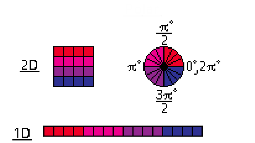
The setup is simple, each probe is evenly spaced within the scene to fit the size of the scene. If our scene is 1024 x 1024 pixel, then for cascade0 each of the 16 x 16 probes are spaced at one probe every 1024/16px or every 64px. These probes then cast their rays out at evenly spaced angles away from each other around the probe as shown in the sample below. Or feel free to download the visual demo source and play around.
How many Cascades?
This is a crucial part of optimization for cascades. You don’t want too many cascades causing performance loss or too few cascades causing radiance field fall-off. This optimization is thankfully easy to implement:
We only need some many cascades up to the point where the ray starting point of the ray interval exceeds the diagonal length of the screen. This is because now rays start to be cast offscreen contributing nothing to the final radiance field.
This max starting interval length can be calculated as this:
// "interval0," is the starting interval at cascade0.
diagonal = sqrt(sqr(width) + sqr(height));
factor = ceil(log4(diagonal/interval0));

// Calculate interval length/start w/ geometric sequences (see next section).
intervalstart = (interval0 * (1.0 - pow(4.0, factor))) / (1.0 - 4.0)
This way for example if we have a screen size of 1920 x 1080 with a diagonal length of 2203px across we calculate the maximum exceeding interval. This length lies outside the screen, so we can take the log4 (because of 4x ray/interval/probe scaling property) and subtract one to find the number of cascades before hitting that interval length:
cascadeCount = ceil(log4(intervalstart)) - 1;Raymarching from Probes
Once cascade layouts are setup the rest is simple raymarching. For each pixel within our cascade we calculate that pixel’s ray index and probe index associated with that pixel in our cascade. Calculating the ray index is simple, we take the pixel’s relative X,Y position within the probe and convert it to a one-dimensional index:
probeX = pixel.x % probeWidth;
probeY = pixel.y % probeHeight;
ray_index = probeY * probeWidth + probeX;
Once we know the ray index calculating the angle is as easy as dividing the index by the total ray count within the probe which is probeWidth x probeHeight, then multiply by 2PI for the angle in radians:
ray_count = probeWidth * probeHeight;
ray_angle = ray_index / ray_count * PI * 2;
The last and final part is satisfying the linear resolution by calculating the length of the ray and how far away the ray should be cast using geometric sequences (generates a number series with a common scaling factor):
// Calculate the interval length/start using geometric sequences.
origin = (interval * (1 - pow(4, cascadeIndex))) / (1 - 4);
length = interval * pow(4, cascadeIndex);
Here the term “interval,” is the initial length of rays in the lowest cascade, cascade0. All of the cascades scale off of the initial settings of cascade0, spacing, angular resolution and starting ray length (interval). Notice how the origin moves 4x further away as we increase the cascade index from 0…N by a power or factor of 4. Going back to tmpvar’s playground we can see a visualization of the interval scaling.
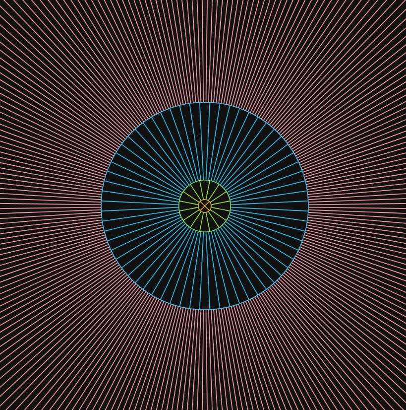
Once we raymarch we can start to see how the cascades all finally come together. The video below is using drastically large interval length of cascade0 to illustrate the scaling between cascades. The gaps between pixels is intentional because those are rays pointing in other directions that did NOT hit a light source or occluder.
Here is that same example with typical ray interval distance.
You can start to see the individual probes as rays of each probe make contact with the light source within the scene. That is still difficult to recognize, so let’s overlay the memory layout with the cascade to tie it together. This is also the best possible way to debug this technique as it helps to visualize and verify that your rays and probes are properly mapped.
I changed the light color to purple for better visualization. With the light at the center you can see how the 1D list of rays and their directions map onto the 2D space of the probes in the cascade texture.
Merging Cascades
This is the (mostly) last piece of the puzzle. Each of our cascades store the linear and angular resolutions which represent the encoded radiance field at any given point along the length of the penumbra. The final goal is to merge our cascades such that they cohesively merge into the final radiance field. This is where Radiance Cascades gets its “infinite rays cast in a finite amount of directions.”
In order to do this we merge our cascades in reverse, starting with the cascade with the highest angular resolution and merging with the cascade above that. However there is no cascade above the final one, so we can start with the one before it. The order then goes: cascadeN-1 merges with cascadeN until we reach cascade0 and merge with cascade1. This merges all of the final radiance into cascade0.
So how does merging work? Remember that each cascadeN+1 has 1/4x probes and 4x rays. This means that in order to merge a lower cascade with a higher cascade, we need to find the 4 nearest probes of cascadeN+1 which match to the current probe within cascadeN. Further for the current ray we match the direction and find the 4 rays pointing in the same direction within each of those 4 probes in cascadeN+1.
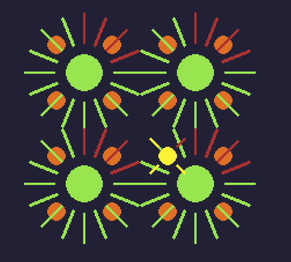
Green being the nearest 4 probes in cascade N+1 to the current ray (red) of the current probe (yellow) in cascade N. Red being the matching ray directions 4:1 between cascadeN and N+1. Once we match the ray directions for each probe we can add up all of the rays for each probe TL (top-left), TR (top-right), BL (bottom-left) and BR (bottom-right).
Since cascade N+1 has lower spatial resolution (less probes at different offsets) the spatial and angular resolution of cascade N+1 doesn’t match that of cascade N. To fix this for any ray of cascade N we find the nearest probes and match 4:1 rays of cascade N+1 and bilinearly interpolate between those probes.
We take the relative X,Y position of the current probe (yellow) between the four upper probes (green) and use that as our “weight,” to determine the spatial and angular resolution to match that of cascade N. If you need a refresher, bilinear interpolation takes four colors, TL, TR, BL, BR as a square and mixes them together. You can see this in action in my Shadertoy example.
This ray interpolation between adjacent probes from upper cascades is where we get our “infinite rays cast from finite directions.” As we cascade down the interpolated angular resolution from higher cascades merges and gets corrected to match the spatial resolution of the next lower cascade and converges to the final radiance field.
Ray Visibility Term and when to Merge
We can’t just “merge,” all of our rays, because some rays in any cascade N+1 may be occluded by some rays in cascade N. This is what the ray visibility term is for. When raymarching instead of storing the alpha value of our raymarched scene, we store whether or not the ray “hit,” the surface (1.0 for hit, 0.0 for no hit):
// On Ray Outside Scene:
if (raypos.x < 0.0 || raypos >= 1.0 || raypos.y < 0.0 || raypos.y >= 1.0) {
    return vec4(0.0, 0.0, 0.0, 0.0);
}

// On Ray Scene Hit:
if (sdf_dist <= EPSILON) {
    return vec4(texture2D(gm_BaseTexture, raypos).rgb, 1.0);
}

// On Ray Outside Interval Range: (end of for loop)
return vec4(0.0, 0.0, 0.0, 0.0);
When merging rays we check the alpha value (ray visibility term), if the term is non-zero we merge rays, if the term is zero we do not merge rays. This is to maintain the penumbra hypothesis. To approximate the penumbra we merge with rays in the above cascade to fill out the missing blurriness or angular resolution in the current cascade and we carry that angular resolution down into the lowest cascade, cascade0.
Screen Space Radiance Field
The final result is simple. We create a render target where its size in pixels is equal to the number of probes in cascade0. This is considered the mipmap of cascade0. Since we merged the cascades in reverse in the previous step cascade0 now contains all of the information both linear and angular to generate the radiance field.
For Each Ray
    Sum up the radiance each ray

Divide the total radiance by the total number of rays.
To generate that mipmap all we do is pass the cascade0 texture into the mipmap shader and for each pixel in the mip-map add up all of the rays associated with that pixel’s probe within cascade0. The final mipmap won’t be the same size as the screen, so you’ll need to scale it up to fit depending on your probe spacing. Enable hardware interpolation and draw the mipmap scaled up to fit the screen. Voila, per-pixel global illumination via Radiance Cascades.
When you visually inspect all of the cascade mip-maps you can then see how each radiance field’s linear and angular resolution is encoded into the final scene.
Notice how the final radiance field for each mip-map contains all of the properties discussed thus far. Higher linear resolution closer to the source, higher angular resolution further from the source.
Conclusion
Radiance Cascades are both simple and complex, but beautiful providing the most efficient possible way that we know to represent per-pixel globally illuminated scenes by taking advantage of the unique properties of the penumbra. This is just a glimpse into the beauty of this technique. If you’d like to play around with the source code (needs some work) see the Github repo for this article!
One of the key things missing from this article is the skybox integral which is included in Fad’s shadertoy example. You can integrate a skybox into RC by merging the sky integral into the highest angular resolution cascade (because skyboxes have little to no linear resolution being extremely far from the “sun”). This does not affect occlusion either so it really does act like an actual skybox! We’ll discuss this in Part Two in detail!
Other things Radiance Cascades can do:
Gravity Simulation by Alexander Sannikov.
3D Screen Space Global Illumination also by Alexander Sannikov.
Volumetrics through high Viscosity Fluids by Mytino.


This is amazing, and very well explained, thank you! I have one question - does this algorithm take view-dependent information into account to also do specular GI? So far it seems to only focus on diffuse GI
I noticed very obvious interference patterns, but it seems that the wavelength of light is not reflected in the algorithm. Why is this?